Electromagnetic Waves
Project
3D Simulation
As of 19 Feb 2024, it is best to run HFSS from a
MOSAIC anywhere redhat linux machine at Mosaic
Anywhere – Mosaic Computing (charlotte.edu) and make sure to
choose the "MATE
(VirtualGL)" or "KDE (VirtualGL)" option when creating a new
session or logging in. Look under the
"Applications>>ElectricalEngineering>>HFSS" menu
(not HFSS mesa) to run the program.
As of 12 Feb 2019, you must run HFSS using Fastx on either
engr-lcs1, engr-lcs2, engr-lcs5, and engr-lcs6. HFSS will now work
on those servers if you choose the "MATE (VirtualGL)" or "KDE
(VirtualGL)" option when logging in with FastX.
As
of 12 Feb 2019, HFSS (an older version that is being
updated) may also be available on MOSAIC
anywhere
Overview
Remain in same project groups for the
semester.
The objective of this project is to simulate coaxial lines using
HFSS software.
NOTE: Use the Project Report Template
IN NO CASE may code or files be exchanged between students, and
each student must answer the questions themselves and do their own
plots, NO COPYING of any sort! Nevertheless, students are
encouraged to collaborate in the lab session.
Part 1
- In this part, you will simulate coaxial lines using HFSS
software.
- Impedance and phase characteristics will be determined.
- Load and run the pulse example as follows:
- Run HFSS from the linux window menu using
Applications::ElectricalEngineering::Ansys HFSS
- If this is the first time you run the software, make a note
of the location of the default directory (perhaps Ansoft or
username/linux/Ansoft) that will be created for your projects
- Store all projects in this directory
- Download the following project file (you may need to hold
down the shift key while you click on the link):
- newer version: mwMetaProj8a.aedt
there is also an older version mwMetaProj8a.hfss
- Move the file into the HFSS directory
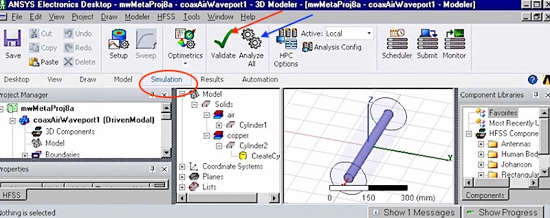
- Load the project from within HFSS using MenuBar::File::Open
(red circle below)
- Double-click the "coaxAirWaveport1" design (red arrow below),
and select the copper cylynder2 (blue arrow below), to see the
corresponding 3D model (yellow arrow below)
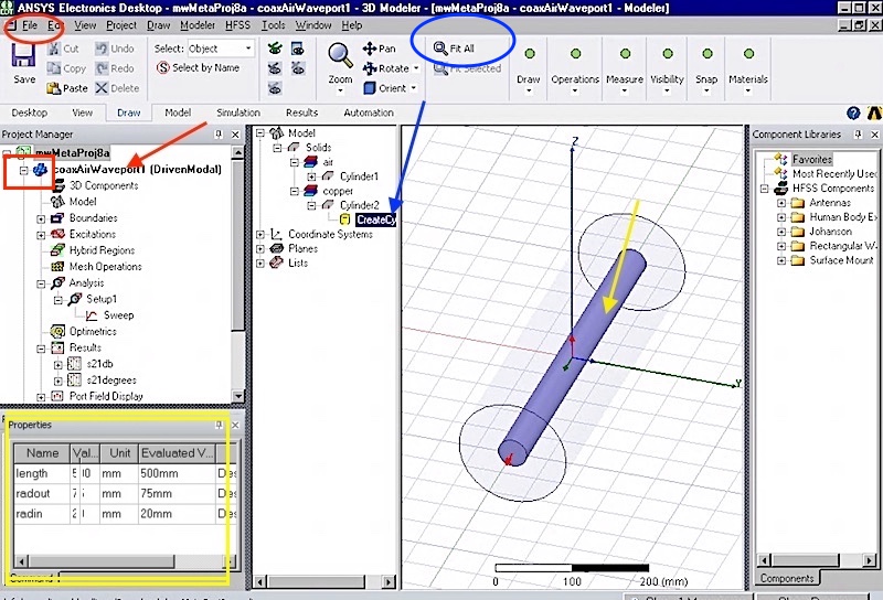
Fig. 001
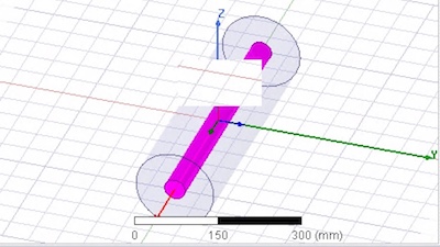
Fig001b
- Press the fitAll button (blue circle above), if the entire 3D
model is not visible
- When you select the cylinder2 item (middle red arrow above),
the corresponding 3D cylinder is highlighted
- Save a snapshot of the 3D model and paste it into your
report.
- Make sure that your
plots, component
values, legends,
axes, and fonts are legible in your report!
- Click the "coaxAirWaveport1" design icon (upper left red box
above) to see the variables used in the design (lower left
yellow box above)
- From the variables, what is the length of the coaxial
line?
- From the variables, what is the radius of the inner conductor
of the coaxial line?
- From the variables, what is the radius of the outer conductor
of the coaxial line?
- Double-click the analysis setup icon (red arrow below) to
observe the setup for the 3D solver
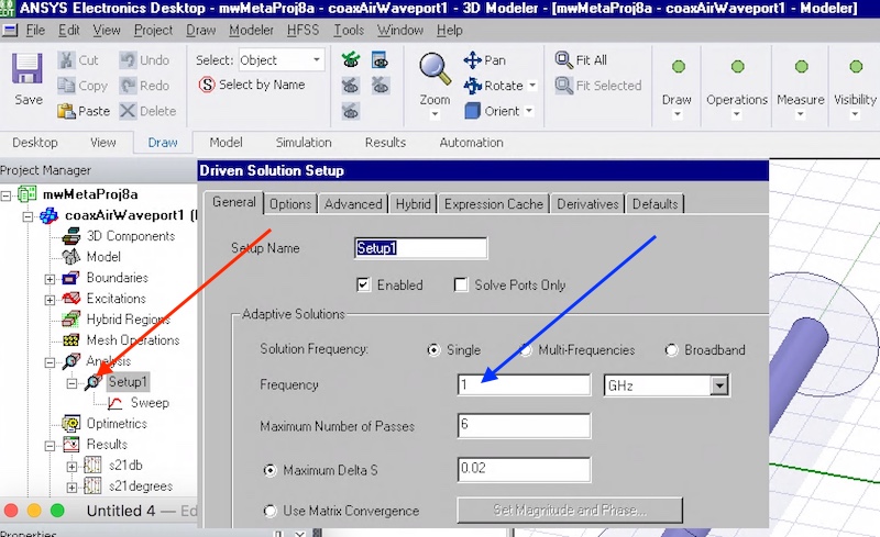
Fig. 002
- From the analysis setup, what is solution frequency (blue
arrow above)?
- Double-click the analysis setup sweep icon (red arrow below)
to observe the setup for the 3D solver
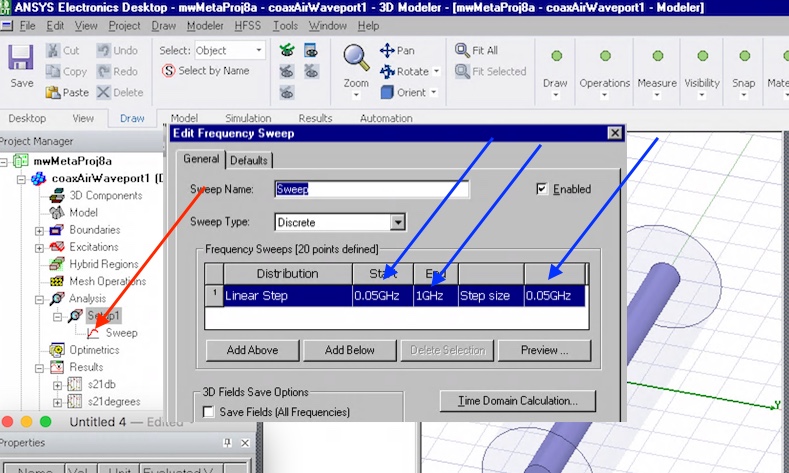
Fig. 003
- From the sweep setup, what are start and stop frequencies
(blue arrows above)?
- Run the simulation
- Select the simulation tab (red circle below)
- validate the design (green arrow below)
- then run the simulation (blue arrows below)
- In the bottom right, during any simulation (if you click the
showProgress button in yellow box at the bottom below), you will
see a progress bar (yellow circle below)
- If your project runs successfully, you should get a message
(red circle below) if you click the showMessages button (in red
box at bottom below) , where message may be such as
- [info] Normal completion of simulation on server:
Local Machine. (8:30:17 PM Feb 04, 2035)
- Observe the magnitude of S21 in dB by double-clicking the
Results::s21dB (red arrow below)
- Observe the phase of S21 in degrees by double-clicking the
Results::s21degrees (blue arrow below)
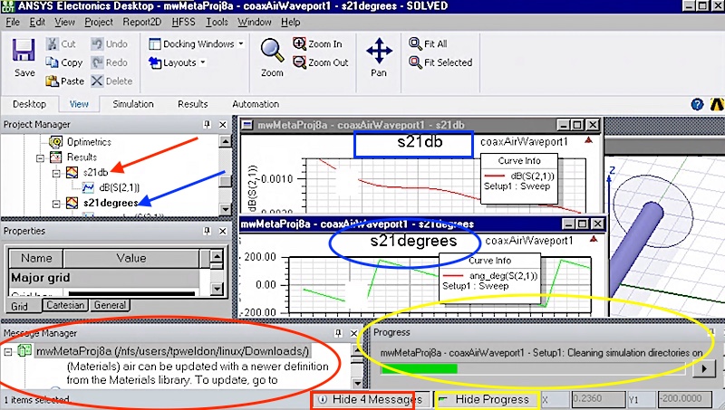
Fig. 004/005
- Save a snapshot of the plot of the angle of S21 in degrees
(yellow rectangle above with heading in red circle ) and paste
it into your report.
- At what frequency is the coaxial line section 90 degrees
long?
- At what frequency would the line length equal a quarter
wavelength in free-space ?
- Observe S21 in dB by double-clicking the Results::s21db (blue
arrow above)
- What is the loss in dB of the coaxial cable at 1 GHz?
- Next, select the results tab (blue arrow below)
- click the solutionsData button (blue circle below)
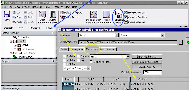
Fig. 006
- Select the matrixData tab (yellow circle above) and check the
Zo box (left yellow arrow above)
- The impedance of the waveport gives the coaxial line impedance
. What is the impedance of the coaxial line (right yellow
arrow above)?
- Next, change the coaxial line material in the outer cylinder
to polyethylene by right-clicking the "air" material (red arrow
below) and selecting "properties"
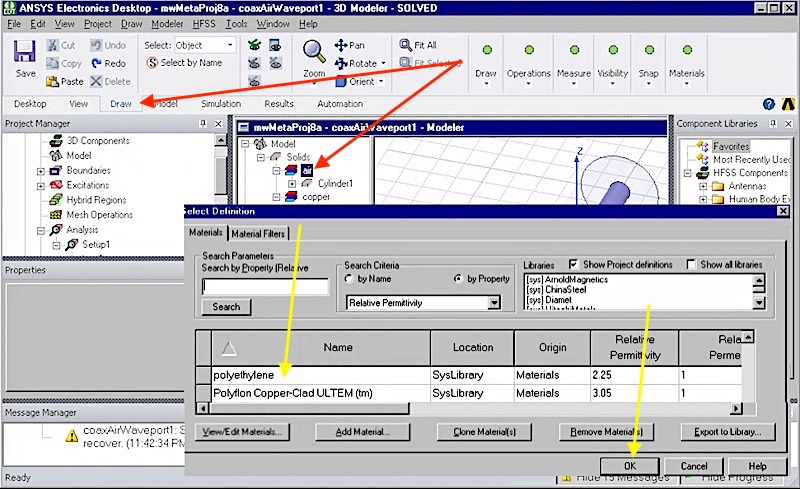
Fig. 007
- In the materials popup, select polyethylene and OK (yellow
arrows above)
- Rerun the simulation as
before, but now with the polyethylene
dielectric and from 0.1 to 1 GHz
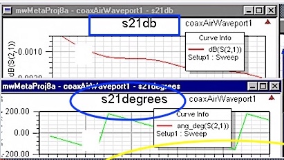 Fig. 008
- For the polyethylene coax,
save a snapshot of the plot of the angle of S21 in degrees
and paste it into your report.
- For the polyethylene coax, save a snapshot of the plot
of S21 in dB and paste it into your
report.
- At what frequency is the polyethylene coaxial line section 90
degrees long?
- Is the previous answer the same frequency where the
polyethylene line length would equal a quarter wavelength in
free-space ?
- Using the same procedure as earlier in this project, what is
the impedance of the polyethylene coaxial cable?
- Identify and highlight "waveport 1" (yellow arrow below)
by selecting "excitation 1" (blue arrow below)
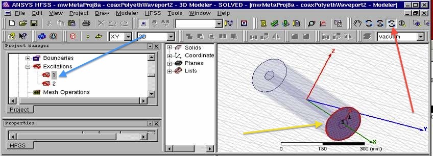
Fig. 009
- As shown above, select the rotateAroundScreenCenter button
(red arrow above), and reorient the 3D model as shown.
- Once you have the model oriented as
shown above, and with the "waveport
1" highlighted as shown above, save a snapshot of
and paste it into your report.
- Exit the program, File->Exit
Report Data
- ============================
WARNING !! ====================================
- **** WARNING **** YOU MUST USE
THE PROJECT REPORT TEMPLATE Below:
- See the Project Report Template at bottom of this page
- A well-written report/paper is
EXPECTED
- STRONGLY RECOMMEND that you read IEEE
authorship series: How to Write for Technical Periodicals
& Conferences
- Clearly describe everything, including:
- variables in block diagrams
- variables in formulas
- units of variables kHz, pF, nH, m, s,
- all traces on plots
- all curves on plots
- all results in any tables
- Minimum required data content for
your report and demos
- Required theory/formulas numbered as
below:
- (1) Coaxial cable formula for characteristic impedance Z0
- Required figures numbered as below:
- Any illegible plots receive zero
credit (must be able to read all numbers, axes, labels,
curves, grids, titles, legends)
- All plots must of professional
quality as in IEEE papers
- LEGIBLE snapshot of the
3D model as in Fig. 001b above, with appropriate caption.
- LEGIBLE For the
polyethylene coax noted below Fig. 007, a plot of S21
in dB from 0.1 to 1 GHz as in Fig. 008, but scaled nicely
- LEGIBLE For the polyethylene
coax noted below Fig. 007, a plot of the phase of S21 in
degrees from 0.1 to 1 GHz
as in Fig. 008, but scaled nicely
- LEGIBLE snapshot of the
waveport as illustrated in Fig. 009 above
- Required tabular data content:
- Table of Fig 001 parameters with 3 columns:
parameter, value, units
- Row 1: length of the coaxial line
- Row 2: radius of the inner conductor of the coaxial line
- Row 3: radius of the outer conductor of the coaxial line
- Row 4: relative permittivity of polyethelene material
between inner and outer conductor of the coaxial line
- Row 5: theoretical impedance of the polyethelene coaxial
line
- Row6: HFSS MatrixData Z0 for polyethelene
simulation (as in Fig 006, but for polyethelene)
See report template below
NOTE ReportTemplate: Use the Project Report Template
YOU MUST ADD CAPTIONS AND FIGURE NUMBERS TO ALL
FIGURES!!
Copyright © 2010-2019 T. Weldon
ANSYS, and HFSS are registered trademarks of ANSYS, Inc. Cadence,
Spectre and Virtuoso are registered trademarks of Cadence Design
Systems, Inc., 2655 Seely Avenue, San Jose, CA 95134. Keysight is a
registered trademarks of Keysight Technologies, Inc. MATLAB and
Simulink are registered trademarks of The MathWorks, Inc. MATHCAD is
a trademark of PTC INC.