Project

Electromagnetic Waves

Project

Time-domain pulse reflections

Overview

Work in assigned project groups.

The objective of this project is to simulate and measure time-domain pulse reflections.

NOTE: Use the Project Report Template

IN NO CASE may code or files be exchanged between students, and each student must answer the questions themselves and do their own plots, NO COPYING of any sort! Nevertheless, students are encouraged to collaborate in the lab session.

Part 1: Measurements

Pulse reflection measurements:

Organize the pulse reflection experiment as shown below

Spring 2019 setup using equipment in open lab area:

Fig 001a

Fig 001b

Fig001c

Connect a 10-dB attenuator to the input of both scope channels as shown above (to create 50 ohm input impedance at the scope).

Also make sure the scope probes are set to 1:1 as shown above.

Set Channel 1voltage scale to 500 mV/div, set Channel 2 at 500 mV/div, and time to 50 ns/div as shown above

Connect the cables as shown with the 25 foot long cable connected between the tee on the pulse generator and the tee on the channel 2 input of the oscilloscope as shown. A shorter cable connects the pulse generator tee to the channel 1 input of the scope.

As shown above, at channel 2 of the oscilloscope, two tees are used to add a pair of 50 ohm terminations in parallel with the channel 2 input 10 dB attenuator. These three 50-ohm impedances effectively terminate the cable in 16.7 ohms when the two terminations are combined in parallel with the 50 ohm attenuator impedance.

Similarly the 50 ohm impedance of the attenuator at scope channel 1 along with the 50 ohm impedance of the signal source, result in a net Thevenin source impedance of 25 ohms driving the long cable.

Set the pulse generator for pulse waveform, 1 MHz frequency, 40 ns pulsewidth, 8.4ns rise/fall time as shown above.

adjust the signal generator amplitude so you have a 2 V peak pulse when the signal generator is connected to channel 1 of the oscilloscope, including the two 10 dB attenuators, and all other terminations/connectors/cables/etc. above Also, adjust the offset voltage of the signal generator so that the baseline of your waveform is at zero volts.

Set the oscilloscope display as above, and the pulses should appear fairly similar to Fig 001b above

Save the plot on a thumb drive for your report, especially noting the peak voltages of the first 2 pulses on each channel

Detach the two 50-ohm terminations from the tee on channel2, and obsrve the reflections on the two wavefoms.

what happened to the reflections and why?

Save the plot without reflections for your report

What is the measured velocity of the pulses in the line, expressed as a fraction of the speed of light, such as 0.4c?

The oscilloscope traces should be nearly the same as your simulation below!

Part 2: Simulation

Start the software:

From a Linux terminal, ADS should be available in the menu (Applications::ElecEngineering::KeysightAdvancedDesignSystem)

From a PC terminal, you must first open a remote Linux session, then proceed as for a Linux terminal

For snapshots use the Linux menu Applications::Graphic::Ksnapshot and select the option to take a legible snapshot of a window rather than a full screen snapshot.

Note: (the following note may not be valid after 2009)

If you find that you have printing problem, see if you have a file ".XprinterDefaults" in your home directory. Move this file to ".XprinterDefaultsOld", and restart ADS ... it will write a new copy of this file that should enable printing.
if this does not work, move your current ".XprinterDefaults" file to ".XprinterDefaultsOld", and try downloading .XprinterDefaults to your home directory. (To download you may need to hold down the "shift key" while you click on the link.) Select the LPDEST printer by File-->PrintSetup-->Options and select Default Printer ($LPDEST) on default_queue

FIRST: create a folder/directory in your home directory named apps and a subfolder in apps named ads

After ADS starts you should get a starting window similar to this (navigate into your apps/ads folder):

Click the help menu item in the upper right (MenuBar::Help) and read through the on-line manuals (see the help tab in ADS), for particular questions it is usually best to use the help index from the ADS window MenuBar::Help to search the manuals.

Note: there might be a bug with the main help items, in that you may need to have a web browser such as fireffox open before help will appear in the browser window .

Load and run the pulse example as follows:

Download the 7zap archive as follows:

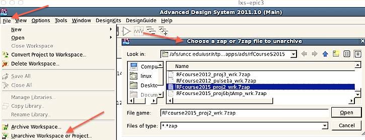
Download the 7zap archive RFcourse2012_pulse1a_wrk.7zap to your ads directory
Use MenuBar::File::Unarchive to extract the project into your ADS directory as follows

You should find a new directory RFcourse2012_pulse1a_wrk created in apps/ads

Run ADS and open the new RFcourse2012_pulse1a_wrk workbook by double-clicking it

Go down through the directory tree to pulse1/schematic and double click that schematic file, and the following schematic should appear. (1 mil = 1/1000 inch)

Double-click the transmission line and look at the variables in the pop-up menu.

Use the mouse to select the variables and observe the changing description at the bottom of the pop-up.

Double-click the "gear" icon (shown below) in the upper right of the window to simulate.

The data plotting window should appear.

Click the "rectangular plot" icon (shown below) in the left of the new popup window to get a plotting grid by dropping the plotting box in the visible area.

In the pop-up window:

Select DataSet -> V1 -> Add
Select DataSet -> V2 -> Add
Select DataSet -> Vsrc -> Add

Click OK at the bottom of the popup

Drop a second plotting box in the visible area, and in the pop-up window:

Select DataSet -> V1 -> Add

Click OK, and the following Time-domain plot should appear.

Save your schematics and plots before exiting ADS

Exit the program, File->Exit.

Change the simulation example to match our lab experiment

Make a copy of the the pulse1/schematic from project 1

Right-click and select "copy cell" to make a copy of this earlier design, and edit it to reflect the new scenario. Replace the "MLIN" transmission line with an appropriate-length TLIND line as shown below (see upper left red arrows below).

For the experiment in the lab, our source impedance will be 25 ohms, our transmission line will be 50 ohms, and our load impedance will be 16.7 ohms. Please note that the voltage listed on the pulse generator in the lab is the matched-load voltage, not open circuit voltage. (Beware: some generators may display the matched-load voltage and some may display the open-circuit voltage) If you are simulating this before your measurements, set the pulse for 0.4 microsecond pulse period, 40 ns wide and 8.4 ns rise/fall , .
Simulate for 500 ns, to see at least one full cycle of the pulse generator.
Based on your measurements in the lab, change the values on the schematic of the voltage source voltage, pulse width, pulse period, etc. and edit the transmission line time delay, such that your final simulation results match your experimental results
Adjust the transmission line delay to better match the delay observed in the lab experiment

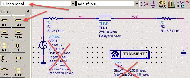
Fig 003

Save a snapshot of your new schematic and paste it into your report.

(SEE BELOW FOR THE REPORT TEMPLATE)

Make sure that your plots, component values, legends, axes, and fonts are legible in your report!
For snapshots use Linux Applications::Graphic::Ksnapshot and select the option to take a legible snapshot of a window rather than full screen

Make sure that your plots, component values, legends, axes, and fonts are legible in your report!

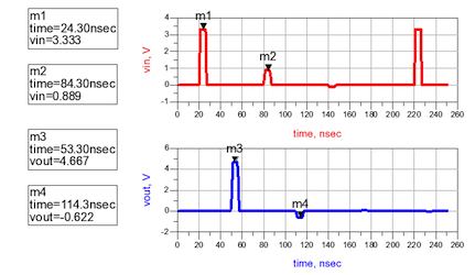
Run the simulation and plot the voltages at the input and output of the transmission line, and add 4 markers to show the pulse voltages of the first two pulses at the input and output of the transmission line as shown below:

Fig 004

Save a snapshot of your input/output pulses as shown above, with markers added, and paste it into your report.

Compute Gamma 1 from the component values on the schematic (reflection coefficient at 1st reflection, at interface between source and transmission line)

Does the simulated voltage agree with your computed reflection coefficient?

Compute Gamma 2 from the component values on the schematic (reflection coefficient at the reflection at far end of line, at the load)

Compute Gamma 3 from the component values on the schematic (reflection coefficient at input, after "round-trip" return)

At the input of the line, for the first pulse reflection, what is the reflection coefficient Gamma1?

At the input of the line, for the first pulse reflection, what is the incident pulse voltage, reflected pulse voltage, and total voltage?

At the output of the line, for the first output, what is the reflection coefficient Gamma2?

At the output of the line, for the first pulse output, what is the incident pulse voltage, reflected pulse voltage, and total voltage?

Save your schematics and plots before exiting ADS

Report Data

============================ WARNING !! ====================================
**** WARNING **** YOU MUST USE THE PROJECT REPORT TEMPLATE Below:

See the Project Report Template at bottom of this page
A well-written report/paper is EXPECTED
STRONGLY RECOMMEND that you read IEEE authorship series: How to Write for Technical Periodicals & Conferences
Clearly describe everything, including:

variables in block diagrams
variables in formulas
units of variables kHz, pF, nH, m, s,
all traces on plots
all curves on plots
all results in any tables

Minimum required data content for your report and demos

Required theory/formulas numbered as below:

(1) Reflection coefficient formula
(2) Total voltage formula

Required figures numbered as below:

Any illegible plots receive zero credit (must be able to read all numbers, axes, labels, curves, grids, titles, legends)
All plots must of professional quality as in IEEE papers

LEGIBLE ADS schematic of the system as in Fig 003 above with delay and loading adjusted to match the measured system, with appropriate caption.
LEGIBLE plot as in Fig 004 of simulated transmission-line input voltage (top) and output voltage (bottom) for the first 4 (2 input, 2 output) pulses
LEGIBLE Photo of measurement setup as in Fig 001a above
LEGIBLE plot in Fig 001b as of measured transmission-line input voltage (top) and output voltage (bottom) for the first 4 (2 input, 2 output) pulses,
LEGIBLE plot in Fig 001b as of measured transmission-line input voltage (top) and output voltage (bottom) for the first for the case with no reflections (both terminations removed from channel 2)

Required tabular data content:

Table of reflection coefficients with 2 columns: particular gamma, theoretical value

Row 1: Gamma1 reflection coefficient at initial input
Row 2: Gamma2 reflection coefficient at initial output
Row 3: Gamma3 round-trip reflection coefficient at input

Table of theoretical and simulated pulse voltages with 3 columns: pulse-name, theoretical voltage, simulated voltage

Row 1: theoretical and simulated pulse voltages at initial input pulse
Row 2: theoretical and simulated pulse voltages at first output pulse
Row 3: theoretical and simulated pulse voltages at second input pulse
Row 4: theoretical and simulated pulse voltages at second output pulse

Table of theoretical and measured pulse voltages with 3 columns: pulse-name, theoretical voltage, measured voltage

Row 1: theoretical and measured pulse voltages at initial input pulse
Row 2: theoretical and measured pulse voltages at first output pulse
Row 3: theoretical and measured pulse voltages at second input pulse
Row 4: theoretical and measured pulse voltages at second output pulse

See report template below

NOTE ReportTemplate: Use the Project Report Template

YOU MUST ADD CAPTIONS AND FIGURE NUMBERS TO ALL FIGURES!!

ANSYS, and HFSS are registered trademarks of ANSYS, Inc. Cadence, Spectre and Virtuoso are registered trademarks of Cadence Design Systems, Inc., 2655 Seely Avenue, San Jose, CA 95134. Keysight is a registered trademarks of Keysight Technologies, Inc. MATLAB and Simulink are registered trademarks of The MathWorks, Inc. MATHCAD is a trademark of PTC INC.