Overview

NOTE: Use the Project Report Template and keep answers to questions on consecutive sheets of paper with all plots at the end.

IN NO CASE may code or files be exchanged between students, and each student must answer the questions themselves and do their own plots, NO COPYING of any sort! Nevertheless, students are encouraged to collaborate in the lab session.

Part 1: Measurements

• In this part, a downconverter is measured
• The downconverter is comprised of a Minicircuits mixer followed by a 10.7 MHz IF filter.  
• The conversion loss is to be measured with LO=100MHz and RF=110.7 MHz. 
  
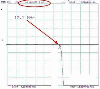
• The response to the image frequency is also to be measured.
• For reference, the IF filter response should be similar to the following:

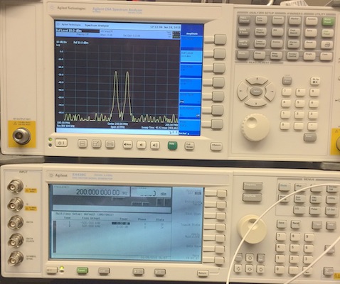
• Test Setup/Station 1
• The test setup for test station 1 is shown below
• The top instrument is an Agilent N1996A spectrum analyzer
  
• The bottom instrument is an Agilent E4438C Vector Signal Generator
  

 

• Use the Agilent E4438C Vector Signal Generator to create the RF signal.  Press “Preset.”  Press “Frequency” 110.7 MHz.  Press “Mod” off,  press “RF” on.  Press “Amplitude” -10 dBm.
• First, connect the cable directly from the signal generator into the spectrum analyzer to check the frequency and power level of the 110.7 MHz input signal. 
• Use a second Agilent signal generator for the 100 MHz LO.   Press “Preset.”  Press “Frequency” 100 MHz.  Press “Mod” off,  press “RF” on.  Press “Amplitude” +7 dBm.
• Connect the IF output to the spectrum analyzer. 
  
• For the Agilent N1996A spectrum analyzer
• Press “Frequency”=10.7 MHz, “span”=10MHz, “Amplitude”=10dBm. 
  
• You should see one tone at 10.7 MHz from IF port. 
  
• Press “Marker,” and “PeakSearch,” 
  
• When you save your first file, check the jpg file on a PC or Sun to make sure it is readable for your report.
• Alternatively, if you are Using an ESA analyzer such as Agilent E4402B, Press “Frequency”=10.7MHz, “span”=10MHz, “Amplitude”=10dBm.  You should see one tone at 10.7 MHz.  Press “Marker,” and “PeakSearch”.   To save a file, use the file menu.  
  
  
• Then, you should observe a spectrum similar to the following

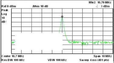
Fig 001

• Press "Marker" and "PeakSearch" to set a marker on the left spectral line 
  
• Record this power level, the input power Pin at 110.7 MHz in dBm, and IF output frequency (10.7 MHz) of the peak (spectrum above). 
  
• Make sure that the marker readout is visible, and you can clearly see the power level and frequency of the peak at the red arrow above, then take a photograph for your report 
  
• Make measurements of image power level and conversion loss at the image frequency of 89.3 MHz
•  Why is the image so strong"
• Make measurements of the output frequency, output power, and conversion loss at the following frequencies (leaving the input power level the same)
• 89.3 MHz
• 89.5 MHz
• 90 MHz
  
• 110 MHz
• 110.5 MHz
• 110.6 MHz
• 110.7 MHz
• 110.8 MHz
• 110.9 MHz
• 111 MHz
• 112 MHz

• In this part, we investigate radio system design using the ADS simulator. .
• For details on radio design concepts, see:
• Superheterodyne receivers, local oscillator, RF, IF, image, image rejection, and mixers
• Noise figure
  
• Load and run the radio receiver design example as follows:
• Download the 7zap archive RFcourse2015_proj15_wrk.7zap  to your ~/apps/ads directory
• Open  the "receiversweep" design, and the following schematic should appear.
  

• Save a snapshot of the schematic for your report.
• Double-click the "gear" icon in the upper right of the window to simulate.
• The data plotting window and 3 plots shown below should appear, as illustrated below.
• The data plotting window and 3 plots shown below should appear, as illustrated below.
  

• Save a snapshot of the 3 plots for your report (as above)
  

• Click the "rectangular plot" icon in the left of the window to drop a plotting box in the visible area, and in the pop-up window:
• Select DataSet -> S(2,1) ->  dB
  
• You should get another sweep of the receiver.
• Double click the plot select "plot options", set the plot x axis to 100 - 105 MHz, and y axis 0 to 80 dB. Then, go to the schematic, double click the S-parameters on the schematic, and set the frequency sweep to 100 - 105 MHz. Rerun the simulation, and note the re-plotted data.

  Print this single plot and turn it in. ( P3 )

• Click the "rectangular plot" icon in the left of the window to drop another plotting box in the visible area, and in the pop-up window:
• Select DataSet -> S(2,1) -> Add  dB
• You should get another sweep of the receiver.
• Double click the plot select "plot options", set the plot x axis to cover the image frequency +/- approx. 1MHz. You should calculate the image frequency, as being "opposite the carrier from the desired signal." 
  
• Then, go to the schematic, double click the s-parameters, and set the frequency sweep to the image frequency +/- approx. 1MHz. Rerun the simulation, and note the re-plotted data. It should look like the following (use the -50 to + 50 dB y-axis scaling).
  

• Save a snapshot of  this single plot as above
  

• What is the image rejection in dB? Hint: difference between desired frequency band and image frequency band levels. 
  
• How does the image rejection compare to the theoretical value from the filter specifications (double-click the filters to see specifications)? 
  
• Why does the image frequency response have the same shape as the frequency response of the desired channel? 
  
• What type of filter is the preselector (Chebyshev, elliptic, Butterworth?).  
  
• What is the gain, Noise Figure in dB, 1dB compression (P1dB in dBm), and output intercept point (OIP3 in dBm) of the first amplifier? 
  

• Use an excel spreadsheet (amp3.xls) to calculate gain, Noise Figure in dB, 1dB compression (P1dB in dBm), and output intercept point (OIP3 in dBm) of the entire radio.
  The spreadsheet results should match your simulation. If the 1 dB compression point is not given for a component, then use Psat (saturation power level) as an approximate 1 dB compression point.

• Optional exercises
  

• Save a copy of the schematic in a differently named file. In this new schematic file, delete the back end of the radio (mixer through IF filter) and connect the output "term" to the output of the second preselector. Sweep the "front end of the radio from 50 to 150 MHz and plot S21. Do not plot unreasonable ranges of dB for the y-axis, rarely would you ever exceed a 120 dB range. 
  

• Return to the original schematic, save another copy, and retune the radio (by changing the LO frequency) to receive at an input frequency of 90 Mhz. Plot the radio frequency response from 40-140 MHz with vertical axis from -50 to 100 dB in steps of 10 dB. 
  
• What is the new LO frequency? 
  
• What is the new Image frequency? 
  
• End of Optional exercises
• 
  
• Save your work!

• See report template below

Report Data

• ============================    WARNING !!    ====================================
  
• **** WARNING **** YOU MUST USE THE PROJECT REPORT TEMPLATE Below:
• See the Project Report Template at bottom of this page
  
• A well-written report/paper is EXPECTED
  
• STRONGLY RECOMMEND that you read IEEE authorship series: How to Write for Technical Periodicals & Conferences
• Clearly describe everything, including:
• variables in block diagrams
• variables in formulas
• units of variables kHz, pF, nH, m, s,
  
• all traces on plots
• all curves on plots
• all results in any tables
  

• Minimum required data content for your report and demos
• Required theory/formulas numbered as below:
• (1) OIP3 formula: OIP3 = Plin + (Plin-P3rd)/2
  
• Required figures:
• Any illegible plots receive zero credit (must be able to read all numbers, axes, labels, curves, grids, titles, legends)
• All plots must of professional quality as in IEEE papers
  
1.  LEGIBLE block diagram of the downconverter that was measured
   
2.  LEGIBLE measured IF spectrum  as in Fig 001 above for 110.7 MHz RF at -10 dBM, with appropriate caption
3. LEGIBLE excel plot of conversion loss from table 1 below
   
4. LEGIBLE ADS radio schematic as in Fig 002
5.  LEGIBLE ADS spectrum plot of desired RF band of 101-102 MHz as in upper left plot of Fig 003 above (must show selectivity)
6.  LEGIBLE ADS spectrum plot of undesired image frequency band as in plot of Fig 004 above (must show selectivity)
• Required tabular data content:
1. Table of measured conversion loss at -10 dBm RF input power with 4 columns: RF input freq in MHz, measured IF output freq in MHz, measured IF output power in dBm, measured conversion loss in dB dBm,
   
• Row 1: 89.3 MHz RF input freq
  
• Row 2: 89.5 MHz MHz RF input freq
• Row 3: 90 MHz MHz RF input freq
• Row 4: 110 MHz MHz RF input freq
• Row 5: 110.5 MHz MHz RF input freq
• Row 6: 110.6 MHz MHz RF input freq
• Row 7: 110.7 MHz MHz RF input freq
• Row 8: 110.8 MHz MHz RF input freq
• Row 9: 110.9 MHz MHz RF input freq
• Row 10: 111 MHz MHz RF input freq
• Row :11 112 MHz MHz RF input freq
2. Table of simulated radio characteristics with 2 columnsL parameter and measured value
• Row1: image rejection in dB
• Row 2: radio gain in dB
  

---

NOTE ReportTemplate: Use the Project Report Template 

  YOU MUST ADD CAPTIONS AND FIGURE NUMBERS TO ALL FIGURES!! 

---

 

---

Copyright © 2010-2018 T. Weldon


ANSYS, and HFSS are registered trademarks of ANSYS, Inc. Cadence, Spectre and Virtuoso are registered trademarks of Cadence Design Systems, Inc., 2655 Seely Avenue, San Jose, CA 95134. Keysight is a registered trademarks of Keysight Technologies, Inc. MATLAB and Simulink are registered trademarks of The MathWorks, Inc. MATHCAD is a trademark of PTC INC.