Overview

NOTE: Use the Project Report Template and keep answers to questions on consecutive sheets of paper with all plots at the end.

IN NO CASE may code or files be exchanged between students, and each student must answer the questions themselves and do their own plots, NO COPYING of any sort! Nevertheless, students are encouraged to collaborate in the lab session.

Part 1: Measurements

• In this part, third-order nonlinearities are measured in the lab.
• Two different test stations are set up in the lab, each station with different equipment and a different amplifier to be measured

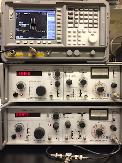
• Test Setup/Station 1
• The test setup for test station 1 is shown below
• The top instrument is an Agilent N1996A spectrum analyzer
  
• The bottom instrument is an Agilent E4438C Vector Signal Generator
  

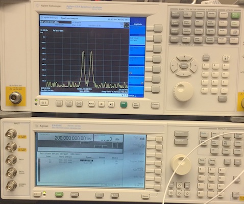
Fig 001

• First, connect the cable directly from the signal generator into the spectrum analyzer to check the frequencies and power levels of the two input signal frequencies.  (The Agilent E4438C Vector Signal Generator is capable of internally creating 2 signals.)
  
• Second, set the signal generator for -25 dBm,  such that you observe two frequencies at 199.5 and 200.5 MHz, each one at a power level of -24 dBm (24 dB below 1 milliwatt) on the spectrum analyzer (red arrow below)  
• If the signals are already present on the spectrum analyzer screen,  only minor adjustments should be needed.  If the instructor is not available, you may need to refer to the detailed setup instructions here
• You should not need to use the following equipment setup information
  
• Detailed instrument setup instructions, if instructor is not available
• First ask the instructor to assist, since minor adjustments are often all that is needed
• Otherwise:
  
• For the Agilent E4438C Vector Signal Generator to create a 2-tone signal for measurement of OIP3. 
  
• Press “Preset.” 
  
• Press “Frequency” 200 MHz. 
  
• Press Mode>More>Multitone>InitializeTable, and select NumberTones=2, FreqSpacing=1MHz, Phase=Fixed, Seed=fixed. 
  
• Press “Mod” on, press “RF” on. 
  
• Press “Amplitude” -20 dBm, “Frequency” 200 MHz, and Mode>more>multitone>mutitoneOn and ApplyMultitone
• For the Agilent N1996A spectrum analyzer
• Press “Frequency”=200MHz, “span”=10MHz, “Amplitude”=10dBm. 
  
• You should see two tones at 199.5 and 200.5 MHz from the signal generator. 
  
• Press “Marker,” and “PeakSearch,” and Marker>more   Add a second marker
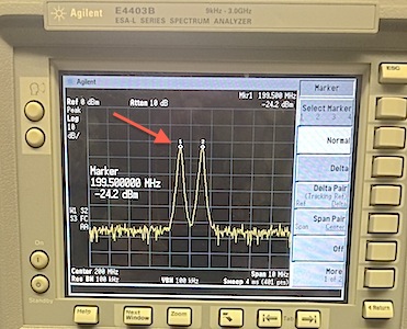
• Make sure that the signal generator is set for -25 dBm
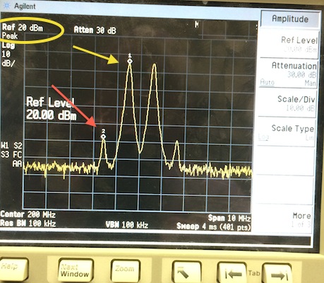
• Then, you should observe a spectrum similar to the following

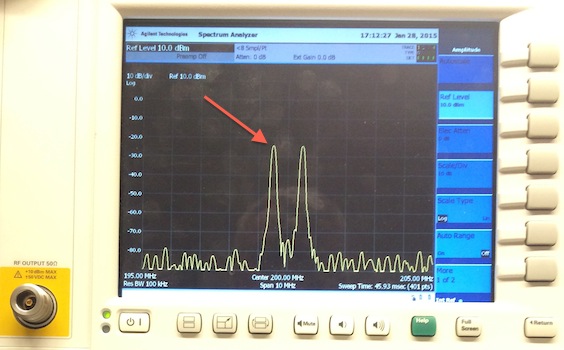
• Press "Marker" and "PeakSearch" to set a marker on the left spectral line (red arrow above)
• The power level should be approximately -29 dBm at 199.5 MHz, 
  
• Record this power level, Pin in dBm, and frequency (199.5 MHz) of the left peak (red arrow above).  The power level that you record here will be the input power level (Pin) to the amplifier that you will measure later
  
• Make sure that the marker readout is visible, and you can clearly see the power level and frequency of the peak at the red arrow above, then take a photograph for your report 
  
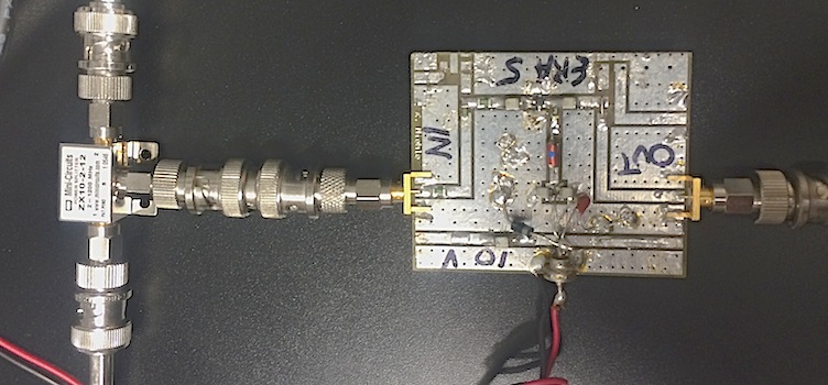
• Connect the MAR-1 amplifier as shown below, with the spectrum analyzer connected to the output and with the signal generator connected to the input and 10Vdc power (red=positive, black=negative)

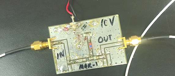
Fig 001

• Recheck to make sure that the signal generator is set for -25 dBm
• You should observe an output spectrum similar to the following

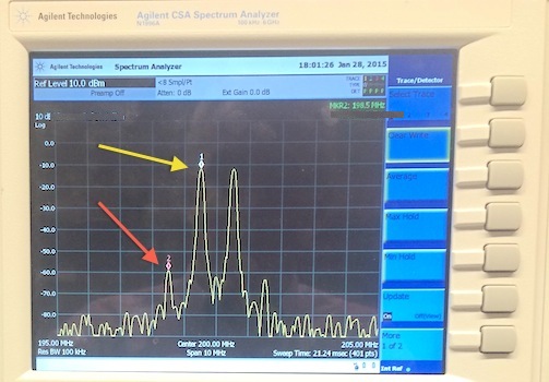
Fig. 002

• Make sure that the marker readout is visible, and you can clearly see the power level and frequency of the peak at the red arrow above, then save a copy for your report (use the USB and save a graphic image with white background) SEE BELOW FOR THE REPORT TEMPLATE
• Record the power level, Pout in dBm, and frequency (199.5 MHz) of the fundamental input frequency left peak (yellow arrow above).  The power level that you record here will be the output power level (Pout) of the amplifier at the fundamental frequency 
  
• The gain of the amplifier is Pout-Pin, .  What is the gain in dB? 
  
• The two third-order distortion frequencies are clearly seen at the left and right of the original input frequencies. 
  
• Record the power level, P3 in dBm, and frequency (198.5 MHz) of the left peak (red arrow above).  
  
• Compute the output third-order intercept point OIP3 from the formula in class: OIP3=Pout + (Pout-P3)/2.  
  

• As discussed in class, if you increase the input power levels by 10 dB, the third order distortion should increase by 30 dB
• Increase the input level from -25 dBm to -15 dBm, and you should see increased distortion similar to the following

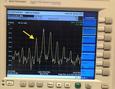
Fig. 003

• Make sure that the marker readout is visible, and make sure that you can clearly see the power level and frequency of the peak at the yellow arrow above, then take a photograph for your report 
  
• Record the power level, P3 in dBm, and frequency (198.5 MHz) of the left peak (yellow arrow above).  
  
• How many dB did the level increase from Q4 to Q6? 
  
• Contact the instructor if the levels do not change by 30 dB
  

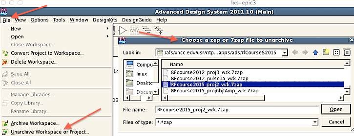
• Download the 7zap archive as follows:
• Download archive RFcourse2015_proj6bjtAmp_wrk.7zap to your ~/apps/ads directory
• Use MenuBar::File::Unarchive to extract the project into your ADS directory as below

• You should find a new directory RFcourse2015_proj6bjtAmp_wrk created in apps/ads
• Run ADS software and open the new RFcourse2012_pulse1a_wrk workbook by double-clicking it
• Go down through the directory tree to ampoip3 and double click that design file,  and the following schematic should appear.

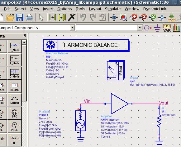
Fig 004

• Save a snapshot of the schematic for your report.  
  
• Make sure that your plots, component values, legends, axes, and fonts are legible in your report!
• For snapshots use the Linux menu Graphics::Ksnapshot and select the option to take a legible snapshot of a window rather than full screen
• Double-click the amplifier symbol on the schematic, and find the TOI parameter, and read the prompt at the bottom of the popup when you select TOI.  What is TOI, and what is its numerical value and units?
  
• Run the simulation
• Harmonic Balance software performs nonlinear simulation that allows the observation of effects such as third-order intermodulation.
• An output showing input and output spectra should appear as follows

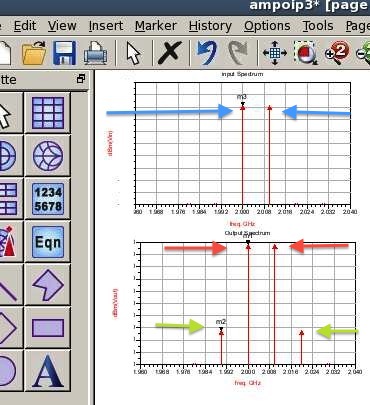
Fig 005

• Save a snapshot of the two spectra as illustrated above, but also with 3 markers added at the 1) leftmost green, 2) leftmost red, and 3) leftmost blue arrows above, and paste the snapshot into your report.   
  
• What are the two frequencies and amplitudes of the input spectrum (blue arrows above)? 
  
• Given the same frequencies and the new amplitudes of the output spectrum, what is the gain of the amplifier from this measurement (amplitude of red arrows above compared to blue arrows above)? 
  
• What are the two frequencies and amplitudes of the third-order products in the output spectrum (green arrows at very bottom above)
  
• Given the data above, what is the measured third order output intercept point, OIP3 in dBm?  
  

Report Data

• ============================    WARNING !!    ====================================
  
• **** WARNING **** YOU MUST USE THE PROJECT REPORT TEMPLATE Below:
• See the Project Report Template at bottom of this page
  
• A well-written report/paper is EXPECTED
  
• STRONGLY RECOMMEND that you read IEEE authorship series: How to Write for Technical Periodicals & Conferences
• Clearly describe everything, including:
• variables in block diagrams
• variables in formulas
• units of variables kHz, pF, nH, m, s,
  
• all traces on plots
• all curves on plots
• all results in any tables
  

• Minimum required data content for your report and demos
• Required theory/formulas numbered as below:
• (1) OIP3 formula: OIP3 = Plin + (Plin-P3rd)/2
  
• Required figures:
• Any illegible plots receive zero credit (must be able to read all numbers, axes, labels, curves, grids, titles, legends)
• All plots must of professional quality as in IEEE papers
  
1.  LEGIBLE Photo of your pc board as in Fig 001 above, with appropriate caption.
   
2.  LEGIBLE measured spectrum plot as in Fig 002 above (must show IP3 components)
3. LEGIBLE measured spectrum plot as in Fig 003 above (must show increased IP3 components)
4. LEGIBLE ADS schematic as in Fig 004
5.  LEGIBLE ADS spectrum plot as in Fig 005 above (must show IP3 components)
• Required tabular data content:
1. Table of measured OIP3 with 3 columns: measured 199.5 MHz power in dBm, measured 198.5 MHz power in dBm, calculated OIP3
   
• Row 1: calculated from your equivalent to Fig 002 above
  
• Row 2: calculated from your equivalent to Fig 003 above (at higher power levels)
  

• See report template below
  

NOTE ReportTemplate: Use the Project Report Template 

  YOU MUST ADD CAPTIONS AND FIGURE NUMBERS TO ALL FIGURES!! 

• Alternate measurement Setup
  
• The test setup for test station 2 is shown below
• The top instrument is an Agilent E4402B spectrum analyzer
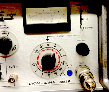
• The bottom instruments are a pair of Racal-Dana signal generators

• First, connect the cable directly from the output of the signal-combiner (connecting the two signal generators) into the spectrum analyzer to check the frequencies and power levels of the two input signal frequencies.  
• Note the signal-combiner in the photo above is used to add the outputs of the 2 signal generators
• Second, set the 2 signal generators for -20 dBm on the dials.  This requires the dials below the meters to be  set to -20 dBm and the vernier dial adjusted for the meter to read "0" on the red scale as below:

• You shuld observe two frequencies at 199.5 and 200.5 MHz, each one at a power level of -24 dBm (24 dB below 1 milliwatt) on the spectrum analyzer (red arrow below).
• If the signals are already present on the spectrum analyzer screen,  only minor adjustments should be needed.  If the instructor is not available, you may need to refer to the detailed setup instructions at the end of this document
• Make sure that the signal generator is set for -20 dBm, as in the picture above
• You should not need to use the following equipment setup information
  
• Detailed instrument setup instructions, if instructor is not available
• First ask the instructor to assist, since minor adjustments are often all that is needed
• Otherwise:
  
• For the Racal-Dana generators, see the photographs and instructions above
• See the photo above for use of the signal-combiner to sum the outputs of the 2 signal generators 
  
• For the Agilent E4402B spectrum analyzer
• Press “Frequency”=200MHz, “span”=10MHz, “Amplitude”=10dBm. 
  
• You should see two tones at 199.5 and 200.5 MHz from the signal generator. 
  
• Press “Marker,” and “PeakSearch,” and Marker>more   Add a second marker
• You should observe a spectrum similar to the following

• Press "Marker" and "PeakSearch" to set a marker on the left spectral line (red arrow above)
• The power level should be approximately -24 dBm at 199.5 MHz, 
  
• Make sure that the marker readout is visible, and you can clearly see the power level and frequency of the peak at the red arrow above, 
  
• Connect the ERA-5 as shown below, with the spectrum analyzer connected to the output and with the signal generator connected to the input and 10Vdc power (red=positive, black=negative)

• See the photo above for use of the signal-combiner to sum the outputs of the 2 signal generators
• Recheck to make sure that the signal generator is set for -20 dBm
• You should observe an output spectrum similar to the following

• Make sure that the reference level on this spectrum analyzer is set to 20 dBm  (yellow circle above)
• Make sure that the marker readout is visible, and you can clearly see the power level and frequency of the peak at the red arrow above,
  
• Perform measurements as in the foregoing first test equipment setup above
•  
  

Copyright © 2010-2018 T. Weldon

ANSYS, and HFSS are registered trademarks of ANSYS, Inc. Cadence, Spectre and Virtuoso are registered trademarks of Cadence Design Systems, Inc., 2655 Seely Avenue, San Jose, CA 95134. Keysight is a registered trademarks of Keysight Technologies, Inc. MATLAB and Simulink are registered trademarks of The MathWorks, Inc. MATHCAD is a trademark of PTC INC.