Overview

NOTE: Use the Project Report Template and  keep answers to questions on consecutive sheets of paper with all plots at the end.

IN NO CASE may code or files be exchanged between students, and each student must answer the questions themselves and do their own plots, NO COPYING of any sort! Nevertheless, students are encouraged to collaborate in the lab session.

Only turn in requested plots ( Pxx ) and requested answers to questions ( Qxx ).

Part 1

Run ADS

Open project5 from the prior project (RFcourse2012_proj5_wrk), open the "receiversweep" design, and the following schematic should appear.

Save a snapshot of the schematic and paste it into your report.    ( P1 )

Make sure that your plots, component values, legends, axes, and fonts are legible in your report!

Double-click the "gear" icon in the upper right of the window to simulate.

The data plotting window and 3 plots shown below should appear, as illustrated below.

Save a snapshot of the 3 plots on one sheet of your report (as above).. ( P2 )

Click the "rectangular plot" icon in the left of the window to drop a plotting box in the visible area, and in the pop-up window:

Select DataSet -> S(2,1) ->  dB
You should get another sweep of the receiver.

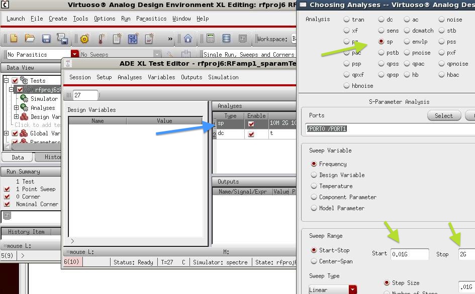
Double click the plot select "plot options", set the plot x axis to 100 - 105 MHz, and y axis 0 to 80 dB. Then, go to the schematic, double click the S-parameters on the schematic, and set the frequency sweep to 100 - 105 MHz. Rerun the simulation, and note the re-plotted data.

Print this single plot and turn it in. ( P3 )

Click the "rectangular plot" icon in the left of the window to drop another plotting box in the visible area, and in the pop-up window:

Select DataSet -> S(2,1) -> Add  dB
You should get another sweep of the receiver.

Double click the plot select "plot options", set the plot x axis to cover the image frequency +/- approx. 1MHz. You should calculate the image frequency, as in the class lecture.  Then, go to the schematic, double click the s-parameters, and set the frequency sweep to the image frequency +/- approx. 1MHz. Rerun the simulation, and note the re-plotted data. It should look like the following (use the -50 to + 50 dB y-axis scaling).

Save a snapshot of  this single plot and turn it in. ( P4 )

What is the image rejection in dB? Hint: difference between desired frequency band and image frequency band levels. (Q1 )

How does the image rejection compare to the theoretical value from the filter specifications (double-click the filters to see specifications)? (Q2 )

Why does the image frequency response have the same shape as the frequency response of the desired channel? (Q3 )

What type of filter is the preselector (Chebyshev, elliptic, Butterworth?). (Q4 )

What is the gain, Noise Figure in dB, 1dB compression (P1dB in dBm), and output intercept point (OIP3 in dBm) of the first amplifier? (Q5 )

Use an excel spreadsheet (amp3.xls) to calculate gain, Noise Figure in dB, 1dB compression (P1dB in dBm), and output intercept point (OIP3 in dBm) of the entire radio, and turn in this spreadsheet. (Q6-Q11 30 points)
The spreadsheet results should match your simulation. If the 1 dB compression point is not given for a component, then use Psat (saturation power level) as an approximate 1 dB compression point.

Save a copy of the schematic in a differently named file. In this new schematic file, delete the back end of the radio (mixer through IF filter) and connect the output "term" to the output of the second preselector. Sweep the "front end of the radio from 50 to 150 MHz and plot S21. Do not plot unreasonable ranges of dB for the y-axis, rarely would you ever exceed a 120 dB range.  Plot this and turn it in. (P5 )

Return to the original schematic, and retune the radio (by changing the LO frequency) to receive at an input frequency of 90 Mhz.
Plot the radio frequency response from 40-140 MHz with vertical axis from -50 to 100 dB in steps of 10 dB. (P6 )

What is the new LO frequency? (Q12 )

What is the new Image frequency? (Q13 )

Part 2

• Download the Cadence file  rfproj6cadence2012.zip 

• Move the file to your ~/cadence6/NCSU16 directory  and extract the file. 
  
• You should see a new library named rfproj6
  
• Fix the links in ~/cadence/NCSU16/cds.lib by opening cds.lib (use the nedit/gedit editor in linux) and editing it to add the lines as before
  
• Run Cadence6

• From library manager, open the RFamp1 cell schematic view in the new rfproj6 library, and you should see a schematic as below
• The 2 PMOS and 3 NMOS transistors in the bias stack on the left (yellow arrows below) are used to set the bias voltages of the differential amplifier components on the right of the schematic
  
• The bottom NMOS in the bias stack is a current mirror that supplies the gate voltage for NMOS current source (red arrow below) of the NMOS differential pair (blue arrows below)
  
• Finally, the two PMOS transistors (purple arrows below) above the differential pair serve as high impedance current-source loads for the differential pair
• Note that the top pair of PMOS transistors (top two yellow arrows below) in the bias stack split the current, just as the pair of PMOS transistors (purple arrows below) at the top of the differential pair split the current from the current source (red arrow below).   Thus, all four PMOS devices have currents that are half the value of the current of the bias stack.
• The bias stack may be thought of as a voltage divider that creates bias voltages from the Vdd power supply.  The bias stack may also be thought of as a current-setting device that established bias currents by virtue of the total current drawn through the devices in series in the bias stack.  To obtain increased current, wider transistors could be used in the bias stack.
  

• Save a snapshot of the schematic as above and paste it into your report.    ( P7 )

• Review of some basic CMOS structures:
• The bias stack consists of a stack of diode-connected FETs

• The basic current mirror structure is as follows:

• The basic differential amplifier structure is:

• In the example circuit in cadence6, RFamp1, the resistors R shown in the above schematic are replaced by the high impedances of the 2 PMOS current mirrors to boost gain (using R=Rds=1/gds of the 2 PMOS devices above the differential NMOS pair)
• Another bias scheme, including input bias and decoupling capacitors is illustrated below:

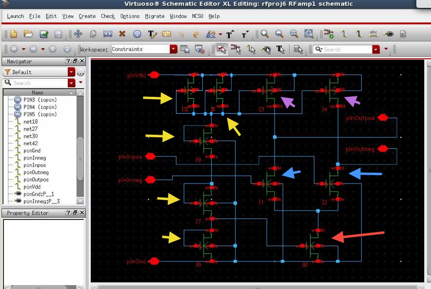
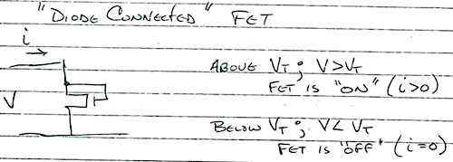
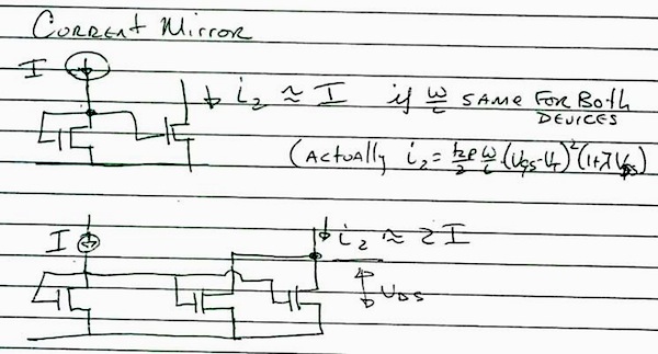
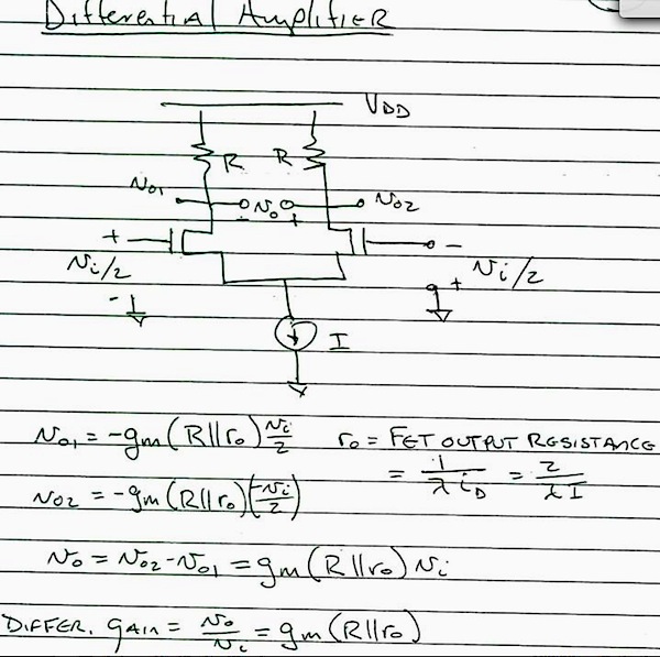
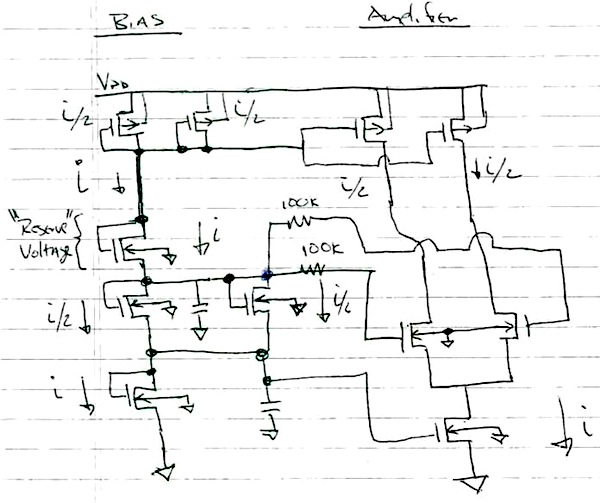
• For a quick review of CMOS theory, see my cmosReview_tpw2011.pdf notes
  

• Next, open the S-parameter test circuit RFamp1_sparamTest, and the schematic should appear as below
  
• Note the two "psin" ports as before (blue arrows below), except that they have 5000 ohm impedance instead of 50 ohms
• The 10,000 ohm resistor and 2.5 volt source (yellow arrows) provide dc bias at the the differential input
  

• Save a snapshot of the schematic as above and paste it into your report (voltage annotations above may be missing).    ( P8 )

• Launch ADE XL using MenuBar::Launch::ADEXL and open the existing view
  
• In ADE XL, right-click the s-parameters (blue arrow below) to edit and observe the simulation settings (green arrows below) as shown below

• Similarly, right click the dc simulation in ADE XL and observe the setup
• Especially note the options button (red arrow below)  and "Save DC operating point" item (left yellow arrow below) and "all" item  (right yellow arrow below) 
• The DC Options window appears after clicking the options button (red arrow below)
  
• The "all" setting and "DC operating point" (yellow arrows below) are needed to later annotate the schematic with dc voltages from simulation
  

• As before, run the simulation (blue arrow below)
• If you get an error regarding the model libraries such as:
• Unable to open input file `/afs/uncc.edu/usr/r/tpweldon/linux/cadence6/ncsu_cdk_160_beta/models/spectre/nom/ami06N.m'
• Then,
  
• you must right-click the test (yellow arrow below) and "OpenTestEditor"
  
• in the TestEditor  run MenuBar::Setup::ModelLibraries
• Delete the offending libraries
• As before, link to your own libraries ~/cadence6/ncsu_cdk_160_beta/models/spectre/nom/ami06N.m and ami06P.m
• 
  

• Select the ADEXL tab and results tab  (black arrows below), if these two tabs are not already selected after simulation runs
  
• After the simulation finishes (blue arrow below), right-click the test (red arrow below), and select Annotate::DCnodeVoltages (yellow arrow below)
• Similarly,  right-click the test (red arrow below) and select Annotate::DcOperatingPoint to add the currents to the schematic, also
  

• The annotated schematic should appear.  Click the schematic tab (blue arrow below) if the schematic does not appear automatically
• The dc voltages (yellow arrows below) should appear on the schematic
• The dc currents of voltage sources (red arrows below) should appear on the schematic

• Save a snapshot of the annotated schematic showing both voltages and currents as above and paste it into your report.    ( P9 )
• What is the dc current supplied to the "pinVdd" pin of the RFamp1 circuit? (Q14 )

• On some cells, the dc voltage annotation will also appear in subcircuit schematics.  However, in most cases this appears not to be true (possible bug).
  
• As shown below, to check the RFamp1 subcircuit, right-click the RFamp1 symbol in the test schematic, and DescendRead (blue arrow below) to see if the voltages were annotated

• Most likely the voltages were not annotated (there seems to be a bug here)
• As a workaround, we can use a slightly different procedure to read the dc voltages
• Right-click the test (red arrow below) and select Print::DCnodeVoltages (yellow arrow below)

• A results display window (red arrow below) should pop up
  
• Click on nodes of the subcircuit (yellow arrows below) and the corresponding dc voltages should be printed in the results window (blue arrows below)
  

• Save a snapshot of theRFamp1 schematic adding all 7 dc node voltages  to the schematic paste it into your report.    ( P10 )

• To plot the S-parameters, click the results browser button (blue arrow below) on the ADE XL toolbar

• In the visualization window that pops up, select the S-parameters, and S11 and S21 (blue arrows below)
• Select default or rectangular and db20 (red arrows below)  to plot the S-parameters in log scale from 0 to 2 GHz
• Change the plot to a white background, and thick lines, one dashed and one solid (yellow arrows below) as shown below
  

• Save a snapshot of the S11 and S21 as above and paste it into your report.    ( P11 )
• x
  

Part 3

• Next, a transient analysis will be done
• Create a new cell schematic view from LibraryManager named RFamp_transientTest in the rfproj6 library
• Enter a schematic as below, with a "vpulse" source (yellow arrow below, from analoglib/sources/independent), two 10,000 ohm resistors (red arrows below), a 2.5 volt dc source, and a 5 volt dc source.
• Add the 4 wire names "vinPos," "vinNeg," "voutPos," "voutNeg" (blue arrows below) by using the toolbar button (black arrow below)
  

• Save a snapshot of the schematic as above and paste it into your report.    ( P12 )

• Select the vpulse, type "q" on the keyboard, and set the vpulse properties as below:

• Launch ADE XL using MenuBar::Launch::ADEXL and create a new view (type adexl)
  
• In ADE XL, click below tests (blue arrow below) to add a new test and open ADE XL test editor
• Click MenuBar::Analysis::Choose  (red arrow below) and setup a transient analysis for 100 ns as shown below.
• As before, use MenuBar::Setup::Models to add the NMOS and PMOS models
• As before, use MenuBar::Session to save your session to cellview
  
• right-click the s-parameters (blue arrow below) to edit the simulation settings (green arrows below) as shown below

• Next, add the outputs using the toolbar button (red arrow below) or MenuBar::Outputs::Setup
• Select the FromSchematic option (blue arrow below)
• Add the four named wires so they appear in the test editor outputs pane (yellow arrows below)
  

• Run the simulation using the RunSimulation button (blue arrow below)
• The plot all the signals using the  PlotAllWaveforms button (red arrow below)

• Plot the four signals from 0 to 100 ns as illustrated in the slightly different plot below in the visualization window
  
• Change the plot to a white background, and thick lines, as shown below

• Save a snapshot of the transient simulation as above (except only for 100 ns)  and paste it into your report.    ( P13 )
• What is the voltage gain (linear ratio vout/vin) of RFamp1 as estimated from the transient simulation?  Hint: use markers to more accurately measure the voltage changes and voltages.   (Q15 )
• What is the voltage gain in dB of RFamp1 from the transient simulation? (Q16 )
• In ADE XL, select the adexl tab, right-click the test, and select Print::DCoperatingPoint
  
• As before, descend through the schematic heirarchy until you reach the bottom level of the schematic hierarchy for one of the differential pair NMOS devices, and observe the transconductance gm as shown below
  

• What is the gm of one of the differential transistors in millisiemens and, assuming the gain = gm*Rload/2 where Rload is your 10,000 ohm differential output load, what do you compute as the theoretical gain? (Q17 )
• If you lower your load to 1000 ohm, you may find the simulation result is closer to theoretical, since other loading effect become relatively smaller

Part 4

• Extract the file in your ADS directory
  
• This ADS example shows you how to use a subcircuit block to make it easy to set up several different tests of your circuit.  This is the best way to test your final project, since changes in the subcircuit are automatically included in all 3 test circuits for ip3, s-parameters, and  transient analysis.
  
• Open the IFamp-sub2-transTest schematic, as below

• Save a snapshot of the schematic and paste it into your report.    ( P14 )
• Run the transient simulation (0-100ns, +/- 1V), and save a snapshot  and paste it into your report.    ( P15 )
• Use MenuBar::Simulate::AnotoateDCvoltage to see the dc bias.  What  is the dc voltage at vinPlus? ( Q18 )
• Select the IFamp-sub2 X1 component, and from the menu bar choose "Push into Hierarchy" (red arrow above) to see the schematic of the subcircuit.  Save a snapshot of the schematic and paste it into your report (not the transistor params at the bottom of the schematic).    ( P16 )
• Double-click the bottom right transistor (MOSFET50).  What is the width and length of the device? ( Q19 )
• Use the menu bar "Pop out" button to return to the top-level schematic.  In the VAR block, what is the value of wp and wn? ( Q20 )
• Open IFamp-sub2-sParamTest  and run the S-parameter simulation (10MHz-1GHz), and save a snapshot  of the S11and S21 rectangular plot and paste it into your report.    ( P17 )
• Save a snapshot  of the Smith chart S11 and S22 rectangular plot and paste it into your report.    ( P18 )
• What is the impedance of the two terms?  ( Q21 )
• Open IFamp-sub2-ip3Test  and run the  simulation, and save a snapshot  of the ip3 plot and paste it into your report.    ( P19 )
• What is the output IP3, OIP3? ( Q22 )
  
• What is the input IP3, IIP3? ( Q23 )
• In the top-level schematic what is the purpose of the BSIM3_Model block? ( Q24 )

Do not add extraneous pages or put explanations on separate pages unless specifically directed to do so. The instructor will not read extraneous pages!

Only turn in requested plots ( Pxx ) and requested answers to questions ( Qxx ). All plots must be labeled P1, P2, etc. and all questions must be numbered Q1, Q2, etc.  YOU MUST ADD CAPTIONS AND FIGURE NUMBERS TO ALL FIGURES!!