Microwave Circuits and
Metamaterials
Project 6
Overview
Remain in same project groups for the
semester.
The objective of this project is to investigate BJT amplifier
design, gain, bandwidth, third-order intercept, and frequency
spectrum using the ADS simulator.
NOTE: Use the Project Report Template and keep answers to questions on consecutive sheets
of paper with all plots at the end.
IN NO CASE may code or files be exchanged between students, and
each student must answer the questions themselves and do their own
plots, NO COPYING of any sort! Nevertheless, students are
encouraged to collaborate in the lab session.
Only turn in requested plots ( Pxx )
and requested answers to questions ( Qxx ).
Part 1
- In this part, the third-order intercept and frequency
spectrum of an amplifier is investigated.
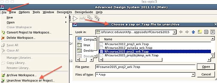
- Load and run the pulse example as follows:
- This project does not seem to function
properly when downloaded as a zip-file, so it must be
downloaded as a 7zap archive as follows:
- Download the 7zap archive RFcourse2015_proj6bjtAmp_wrk.7zap
to your ~/apps/ads directory
- Use MenuBar::File::Unarchive to extract the project into
your ADS directory as below
- This zip-file does not function
properly when downloaded, use 7zap above: Download
the following zip-file (you may need to hold down the shift
key while you click on the link):
RFcourse2015_proj6bjtAmp_wrk.zip
- Move the zip-file into the apps/ads directory, and extract
it
- You should find a new directory
RFcourse2015_proj6bjtAmp_wrk created in apps/ads
- Run ADS software and open the new RFcourse2012_pulse1a_wrk
workbook by double-clicking it
- Go down through the directory tree to ampoip3 and double click
that design file, and the following schematic should
appear.
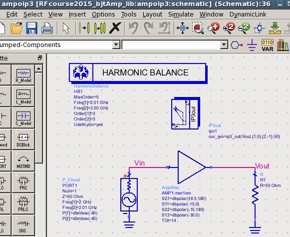
- Save a snapshot of the schematic and paste it into your
report. ( P1 )
- Make sure that your
plots, component
values, legends,
axes, and fonts are legible in your report!
- For snapshots use the
Linux menu Graphics::Ksnapshot and select the option to
take a legible snapshot of a window rather than full screen
- Double-click the amplifier symbol on the schematic, and find
the TOI parameter, and read the prompt at the bottom of the
popup when you select TOI. What is TOI, and what is its
numerical value and units? ( Q1 )
- Run the simulation
- Harmonic Balance software performs nonlinear simulation that
allows the observation of effects such as third-order
intermodulation.
- An output showing input and output spectra should appear as
follows
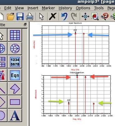
- Save a snapshot of the two spectra as illustrated above, but also with 3 markers added at the
1) leftmost green, 2) leftmost red, and 3) leftmost blue arrows
above, and paste the snapshot into your
report. ( P2 )
- What are the two frequencies and amplitudes of the input
spectrum (blue arrows above)? ( Q2 )
- Given the same frequencies and the new amplitudes of the
output spectrum, what is the gain of the amplifier from this
measurement (amplitude of red arrows above compared to blue
arrows above)? ( Q3 )
- What are the two frequencies and amplitudes of the third-order
products in the output spectrum (green arrows at very bottom
above) ( Q4 )
- Given the data above, what is the measured third
order output intercept point, OIP3 in dBm? Show your
formula, numbers, and calculation ( Q5 )
Part 2
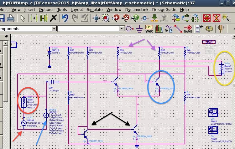
- In this part, the gain and bandwidth of a BJT differential
amplifier is investigated.
- What are the source and load impedances, Term1 (red circle
above) and Term2 (yellow circle above) ? (
Q6 )
- The ac voltage source (red arrow above) is used for ac sweep
simulation, and it acts as a short circuit for other
simulations, since it is a voltage source.
- The pulsed current source (blue arrow above) is used for
transient simulations, typically to assure stability. It
becomes an open circuit during other simulations, since it is a
current source.
- What is the role of the pair of transistors beneath the two
black arrows above? ( Q7 )
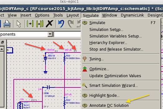
- Run the simulation and annotate the the dc voltages and
currents (yellow arrow below) and the bias should appear (red
arrows below)
- What is the dc bias current to the right-side BJT in the
differential amplifier (blue circle above) ? ( Q8 )
- What is Vce across the BJT in the blue circle, and what is the
voltage across the collector resistor directly above the BJT? ( Q9 )
- What is the highest voltage at the collector of the BJT in the
blue circle when it is turned off (no current), and what is its
lowest collector voltage when all the available current from the
current source flows through the BJT in the blue circle?
This provides an estimate of maximum voltage swing. ( Q10 )
- Save a snapshot of the annotated
schematic and paste it into your report. ( P3 )
- When the simulation completes you should see a variety of
plots as illustrated below
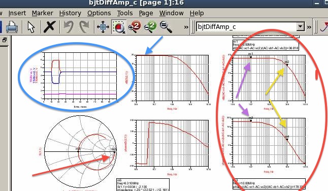
- In the ac sweep differential gain and phase plots (red circle
above) set the two left markers (purple arrows above) at 2
MHz to measure the low-frequency gain and phase, and set the two
right markers (yellow arrows above) to the 3 dB and 45 degree
phase points. After positioning the
markers (yellow arrows above), paste
the 2 plots (red circle above)
into your report as a single figure as illustrated in the red
circle above. ( P4 )
- Adjust the low-frequency marker on the Smith chart to 1
MHz. After positioning the markers,
paste the Smith chart plus markers into your
report. ( P5 )
- What is the 3 dB bandwidth and unity-gain bandwidth (frequency
at which gain falls below unity) of the amplifier (you must use plots in red circle above)?
( Q11 )
- What is the amplifier gain in dB at 2 MHz (you must use plots in red circle above)?
( Q12 )
- We will next need to determine the BJT operating point to
calculate the gain, so:
- Select the right-side BJT in the differential pair (lower
purple circle below) and push into the hierarchy (upper purple
circle below)
- In the schematic model for the BJT, select detailed
operating point (blue arrow below) and click on the BJT (blue
circle below)
- You should see the operating point data (red circle below)
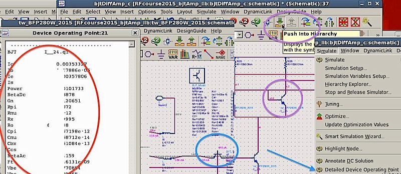
- The collector current should be about 3 mA as shown above.
Take a snapshot of the operating point, and paste it into your
report. ( P6 )
- Compare the value of gm in the operating point printout with
the theoretical value gm=Ic/Vt on page 17 of Review of CMOS and BJTs
. ( Q13 )
- Compare the value of Rpi with the theoretical value of
Rpi=beta/gm on page 17, and state whether the input impedance on
the Smith chart measured above equals 2*Rpi ( Q14 )
- Using the formula on page 19 and the value of Ro from your
printout, what is the ideal gain in dB (be careful with dB here,
since gain is in volts-per-volt) ( Q15 )
- Since half of the resistance of Term2 is also in parallel with
R and Ro, recompute your answer to the previous question
including this added effect, and compare your new re-calculated
gain in dB with the dB gain measured at 2 MHz in your ac sweep.
( Q16 )
Part 3
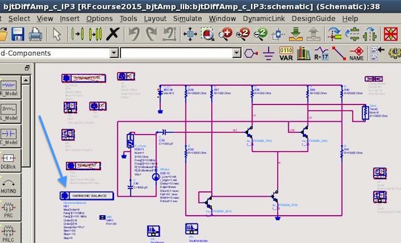
- Go down through the directory tree to bjtDiffAmp_c_IP3 and
double-click that design file, and the following schematic
should appear, with a Harmonic Balance simulation (blue arrow
below)
- Harmonic Balance software performs nonlinear simulation that
allows the observation of effects such as third-order
intermodulation.
- Start the simulation, and you should get a plot of linear
output power versus input power (blue curve below)
superimposed with a plot of third-order nonlinear output power
versus input power (red curve below) as follows
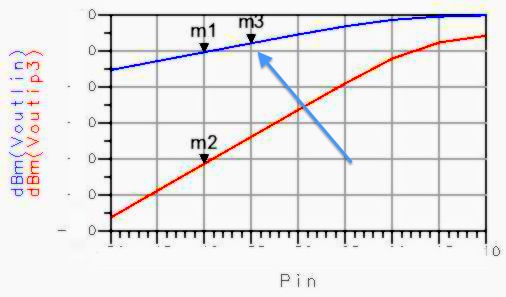
- Move marker m3 (blue arrow above) to the point of 1 dB
gain compression, and leave the other 2 markers located as shown
above. After positioning the
markers, paste the plot into your report. ( P7 )
- Note that marker m1 indicated the output power (red arrows
below) of the two fundamental input frequencies, ...as again
shown below for convenience. The marker m2 corresponds to
the power level of the two third-order spectral components at
the amplifier output (green arrows below). The x-axis
denotes the power level of the input spectral components (blue
arrows below)
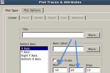
- Modify the plot axes so that you can extend the two curves to
find the intercept point graphically, just double-click the plot
and adjust axes as follows
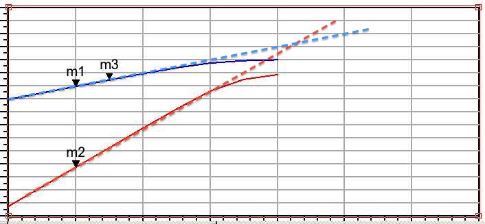
- Then, graphically plot the extended lines as illustrated below
and elsewhere
- Save a snapshot of the extended plots
as illustrated above, and paste it into your
report. ( P8 )
- From the graph, what are the input third order intercept
point, IIP3, and output
third order intercept point, OIP3, in dBm? ( Q17 )
- Save your work!
NOTE ReportTemplate: Use the Project Report Template
and keep answers to questions on
consecutive sheets of paper with all plots at the end.
Do not add extraneous pages or put explanations on separate
pages unless specifically directed to do so. The instructor will
not read extraneous pages!
Only turn in requested plots (Pxx )
and requested answers to questions (Qxx ).
All plots must be labeled P1, P2, etc. and all questions must be
numbered Q1, Q2, etc. YOU MUST ADD CAPTIONS AND FIGURE
NUMBERS TO ALL FIGURES!!
Copyright 2010-2015 T. Weldon
Cadence, Spectre and Virtuoso are registered trademarks of
Cadence Design Systems, Inc., 2655 Seely Avenue, San Jose, CA
95134. Agilent and ADS are registered trademarks of Agilent
Technologies, Inc.