Microwave Circuits and Metamaterials

Project 3

Overview

Remain in same project groups for the semester.

The objective of this project is to measure S-parameters and pulse reflection in the lab.

NOTE: Use the Project Report Template and keep answers to questions on consecutive sheets of paper with all plots at the end.

IN NO CASE may code or files be exchanged between students, and each student must answer the questions themselves and do their own plots, NO COPYING of any sort! Nevertheless, students are encouraged to collaborate in the lab session.

Only turn in requested plots (Pxx ) and requested answers to questions (Qxx ).

Part 1

In this part, S-parameters and pulse reflections are measured in the lab.
There will be two stations in the lab, one for pulse measurements and one for S-parameter measurements.
Due to limited space, please alternate in groups of 2 at each station to perform the experiments.
For expedience, each student should take pictures of the displays to include in your reports. If you dont have access to a cameraphone/etc, ask me to take a picture for you when you are ready, and i can email it to you.

Pulse reflection measurements:

We will be making a pulse reflection measurement that roughly corresponds to our simulation experiments in the pulse1/schematic from project 1
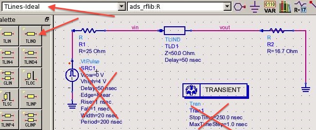
Right-click and select "copy cell" to make a copy of this earlier design, and edit it to reflect the new scenario. Replace the "MLIN" transmission line with an appropriate-length TLIND line as shown below (see upper left red arrows below).
For the experiment in the lab, our source impedance will be 25 ohms, our transmission line will be 50 ohms, and our load impedance will be 16.7 ohms. Please note that the voltage listed on the pulse generator in the lab is the matched-load voltage, not open circuit voltage. If you are simulating this before your measurements, set the pulse for 5 MHz pulse frequency, 20 ns pulsewidth, 5ns rise/fall time.
Simulate for 250 ns, to see at least one full cycle of the pulse generator.
Based on your measurements in the lab, change the values on the schematic of the voltage source voltage, pulse width, pulse period, etc. and edit the transmission line time delay, such that your final simulation results match your experimental results

Save a snapshot of your new schematic and paste it into your report. ( P1 )

Make sure that your plots, component values, legends, axes, and fonts are legible in your report!

For snapshots use the Linux menu Graphics::Ksnapshot and select the option to take a legible snapshot

Run the simulation and plot the voltages at the input and output of the transmission line, and add 4 markers to show the pulse voltages of the first two pulses at the input and output of the transmission line as shown below:

Save a snapshot of your input/output pulses as shown above, with markers added, and paste it into your report. ( P2 )

At the input of the line, for the first pulse reflection, what is the reflection coefficient Gamma1? ( Q1 )

At the input of the line, for the first pulse reflection, what is the incident pulse voltage, reflected pulse voltage, and total voltage? ( Q2 )

At the output of the line, for the first output, what is the reflection coefficient Gamma2? ( Q3 )

At the output of the line, for the first pulse output, what is the incident pulse voltage, reflected pulse voltage, and total voltage? ( Q4 )

Organize the pulse reflection experiment as shown below

Make sure that channel1 and channel2 of the oscilloscope are set to 50 ohm input impedance.

Connect the cables as shown with the 18 foot long cable connected between the tee on the pulse generator and the tee on the channel2 input of the oscilloscope. A shorter cable connects the pulse generator tee to the channle1 input of the scope.

At channel2 of the oscilloscope, two tees are used to add a pair of 50 ohm terminations in parallel with the channel2 input. These three 50-ohm impedances effectively terminate the cable in 16.7 ohms when the two terminations are combined in parallel with the 50 ohm scope impedance.

Similarly the 50 ohm impedance of scope channel1 acts as a voltage divider in series with the 50 ohm impedance of the signal source, resulting in a net Thevenin source impedance of 25 ohms.

Note that the pulse voltage of the pulse generator is rated into a matched load.

Set the pulse generator for 2 V max, 0 V min, 5 MHz frequency, 20 ns pulsewidth, 5ns rise/fall time.

Set the oscilloscope display as follows, and the pulses should appear similar (not the same) as below:

Detach the long cable from the tee at the pulse generator, what is the voltage when only the 50 ohm oscilloscope as a load. ( Q5 )

Reattach the long cable and save a cellphone picture of your measured input (top) and output (bottom) pulses as shown above ( P3 )

What is the measured velocity of the pulses in the line, expressed as a fraction of the speed of light, such as 0.4c? ( Q6 )

The oscilloscope traces should be nearly the same as your simulation!

S-parameter measurements:

We will be making S-parameter measurements that roughly correspond to a situation similar to our project 2 simulation.
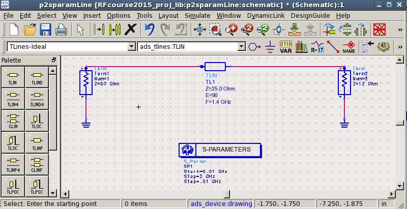
Open the p2sparamLine design in the workbook by clicking that design file.

Right-click and select "copy cell" to make a copy of this earlier design, and
Edit the new copy so that it reflects the scenario in the lab. Change the TLIN line to 50 ohms with E=90 at whatever frequency in MHz best corresponds to your lab measurements, set source Term1 to 50 ohms, and load Term2 to 25 ohms. Change the S-parameter sweep to go from 1 to 50 MHz in 1 MHz steps. Adjust to an appropriate-length the TLIND line such that it reflects your measurements using the the approximately 6-foot long line in the lab (if you want to estimate it before going into the lab, assume a velocity of 0.7 c, and length of 6 feet).
Save a snapshot of your new schematic and paste it into your report. ( P4 )

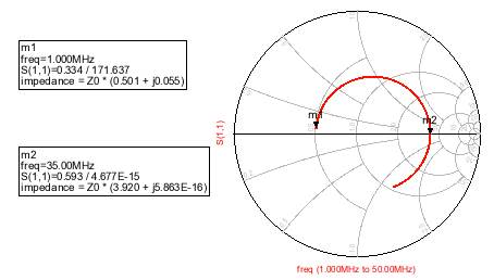
Run the simulation, and plot the Smith chart (somewhat different from that illustrated below):

Set two markers as above (one at 1 MHz and the other at where it crosses the axis on the right side)
Save a snapshot of the schematic and paste it into your report. ( P5 )
What are the two un-normalized impedances (assume closest pure resistance) at the markers, and what is the transformer ratio (ratio of the 2 impedances)? ( Q7 )

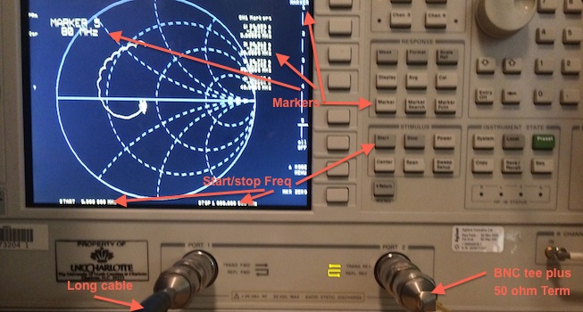
Set up the S-parameter measurement as illustrated below, with a bias tee and 50-ohm term at port 2 to create the 25 ohm load

Have the instructor adjust the display to the following format:

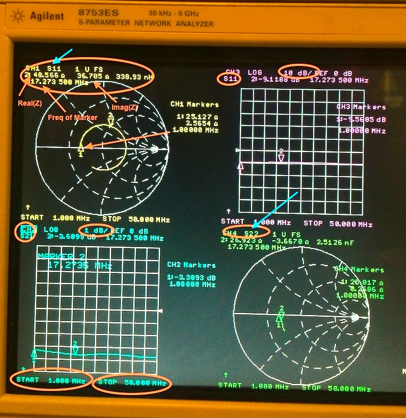
Check that the start/stop are 1 MHz and 50 MHz (bottom left above), and that the two Smith charts are S11 and S22 (blue arrows above)
Adjust marker1 to 1 MHz, and adjust marker2 to where the plot crosses the Smith chart on the right (as shown in the simulation above). See the arrows in the previous photograph for the location of the marker controls.
Save a cellphone picture of the netwrok analyzer display as above (but with markers correctly positioned) and paste it into your report. ( P6 )
What are the two un-normalized impedances (assume closest pure resistance) at the tow markers, and what is the transformer ratio (ratio of the 2 resistances)? ( Q8 )
Compute reflection coefficient Gamma, and return loss seen from port1 at 1MHz (assume the transmission line is a wire). ( Q9 )
From the upper right plot of S11 in dB, what is the measured S11 in dB at 1 MHz? ( Q10 )
Why do you "see a circle" on the Smith chart of S11, but not on the Smith Chart of S22? ( Q11 )

Report

NOTE ReportTemplate: Use the Project Report Template and keep answers to questions on consecutive sheets of paper with all plots at the end.

Do not add extraneous pages or put explanations on separate pages unless specifically directed to do so. The instructor will not read extraneous pages!

Only turn in requested plots (Pxx ) and requested answers to questions (Qxx ). All plots must be labeled P1, P2, etc. and all questions must be numbered Q1, Q2, etc. YOU MUST ADD CAPTIONS AND FIGURE NUMBERS TO ALL FIGURES!!

Cadence, Spectre and Virtuoso are registered trademarks of Cadence Design Systems, Inc., 2655 Seely Avenue, San Jose, CA 95134. Agilent and ADS are registered trademarks of Agilent Technologies, Inc.